How to Format a Cell in Excel: Complete Guide

Excel is basically a calculator wearing a suit. And cell formatting is the tie. Sure, the math still works without it,
but nobody wants to stare at a spreadsheet that looks like it just rolled out of bed.

In this complete guide, you’ll learn exactly how to format a cell in Excelfrom quick Ribbon tricks to the mighty
Format Cells dialog boxplus practical examples, troubleshooting tips, and real-world formatting “war stories”
(the safe kind… mostly involving missing dollar signs).

What cell formatting really does (and what it definitely doesn’t)

Cell formatting controls how values look, not what they actually are. For example, you can format
0.5 to display as 50%, but the stored value is still 0.5.
This is why formatting is powerful: it makes data readable without breaking calculations.

Formatting can change appearance through number formats, fonts, colors, borders, alignment, and more.
But it won’t magically fix messy data. (It can only make messy data look more confident.)

The fastest ways to format a cell in Excel

There are three main routes, depending on whether you want “quick and simple” or “I need every setting known to humankind.”

1) Use the Home tab (quick formatting)

Select a cell (or range), then use the Home tab to adjust:
Number formats, Font, Alignment, Wrap Text,
Fill Color, and Borders.
This is perfect for everyday spreadsheet cleanup.

2) Right-click (surprisingly powerful)

Right-click a cell for options like Format Cells, quick number formatting shortcuts, and paste options.
If you’re a right-click person, Excel respects your lifestyle.

3) Open the Format Cells dialog box (the “control center”)

For full control, open Format Cells. On Windows, the famous shortcut is Ctrl + 1.
On Mac, it’s commonly Command + 1.

Inside this dialog, you’ll typically find tabs like:
Number, Alignment, Font, Border,
Fill/Patterns, and Protection.
This is where Excel keeps the “advanced settings” that the Ribbon can’t fully show.

Number formatting: make your data instantly readable

Number formatting is often the most important cell formatting skill because it prevents misunderstandings.
A plain 1000000 can be a million dollars… or a million jellybeans. Formatting clarifies intent.

Common built-in number formats

• General: Excel’s default “figure it out” mode.
• Number: Choose decimal places and separators (like commas).
• Currency and Accounting: Great for money (Accounting aligns symbols neatly).
• Percentage: Displays decimals as percentages (0.25 becomes 25%).
• Date and Time: Displays date/time in readable formats.
• Scientific: Useful for very large/small values.
• Text: Treats content as text (helpful for IDs, codes, and “numbers that shouldn’t do math”).

Step-by-step: format numbers, currency, and dates

1. Select the cells you want to format.
2. Open Format Cells (Ctrl + 1 on Windows).
3. Go to the Number tab.
4. Pick a category (Number, Currency, Date, etc.), then adjust options like decimal places or symbols.
5. Click OK.

Custom number formats: the secret weapon

Built-in formats are greatuntil you want something specific, like:
“Show negatives in red,” “Add ‘kg’ after weights,” or “Display phone numbers with leading zeros.”
That’s where Custom formats shine.

Where to find it: Format Cells → Number tab → Category: Custom

Custom format basics (the characters that matter):

• 0 = required digit (shows 0 if empty)
• # = optional digit (shows nothing if empty)
• ? = digit placeholder (helps align decimals/fractions)
• @ = text placeholder

Example 1: add text after a number

If a cell contains 12, it displays as 12 kg. The value is still 12,
so formulas still work.

Example 2: show thousands with a K

25300 displays as 25.3K. Great for dashboards where space is tight.

Example 3: format positives, negatives, and zeros differently

This uses sections separated by semicolons: positive ; negative ; zero.
You can even add a fourth section for text.

Example 4: preserve leading zeros (IDs, ZIPs, codes)

If you type 123, it displays as 00123. Handy for ZIP codes, product SKUs, and anything that should stay a fixed length.
(Pro tip: if you never want Excel to treat it as a number, format the cell as Text first.)

Format text in cells: fonts, emphasis, and readability

Text formatting includes bold/italic, font size, font color, and effects. It’s useful when you want headings to stand out,
totals to look official, or a warning label to politely yell at the reader.

Best practice: keep it consistent. One spreadsheet with five fonts feels like five spreadsheets arguing in a group chat.
Use bold for headers, subtle color for categories, and save neon colors for true emergencies.

Quick moves that make a sheet look “finished”

• Bold the header row
• Use a slightly larger font for section titles
• Apply a consistent number format to numeric columns
• Use a light fill color for input cells (so people know what to edit)

Alignment and layout: where Excel goes from “data” to “document”

Wrap text (so your cells stop cutting off sentences)

When text is too long, you can wrap it so it appears on multiple lines in the same cell.
This is great for notes, addresses, or column headers that would otherwise stretch your sheet into the next time zone.

1. Select the cell(s).
2. Home → Alignment group → Wrap Text.

Want a manual line break inside a cell? In many Excel setups on Windows, Alt + Enter inserts a new line.

Merge cells (use carefully)

Merging cells is common for big titles, but it can cause headaches with sorting, filtering, and selecting ranges.
Also, when you merge multiple cells, Excel keeps the content from only one cell and discards the rest.
Use it sparinglymostly for presentation areas, not raw datasets.

AutoFit column width and row height

If you see ##### in a cell, it often means the column is too narrow to display the value.
AutoFit fixes this quickly:

• Double-click the boundary between column letters (like between A and B) to AutoFit.
• Or use Home → Cells → Format → AutoFit Column Width / AutoFit Row Height.

Borders and fill color: structure without chaos

Borders and shading help guide the eyewhen used with restraint. A clean spreadsheet uses borders like a map uses roads:
enough to navigate, not so many that you can’t see the land.

Simple border strategy that works almost everywhere

• Use a thick outside border for a table area
• Use thin inside borders if needed for readability
• Avoid heavy borders on every single cell unless you enjoy visual static

Cell styles: consistent formatting you can reuse

Cell Styles are preset formatting bundles (font + fill + borders + number format).
They’re perfect when you want consistency: titles, headers, input cells, totals, warnings, and more.

You can also create a custom style for your workbooklike “Inputs,” “Outputs,” “Totals,” or “Do Not Touch Unless You Like Trouble.”
The big advantage: if you update a style, every cell using that style updates too.

How to apply a style

1. Select the target cells.
2. Home → Styles group → Cell Styles.
3. Choose a style (or create your own).

Conditional formatting: formatting that reacts to your data

Conditional formatting automatically applies formatting based on ruleslike highlighting duplicates, flagging overdue dates,
or adding data bars to show magnitude. It’s “set it once, let Excel watch the data” energy.

Popular conditional formatting rules

• Highlight Cells Rules: greater than, less than, between, text contains, dates occurring
• Top/Bottom Rules: top 10 items, bottom 10%, above average
• Data Bars, Color Scales, and Icon Sets for quick visual analysis
• Duplicate Values: instantly spot repeats

Example: highlight duplicates in a list

1. Select the list (e.g., column of invoice numbers).
2. Home → Conditional Formatting → Highlight Cells Rules → Duplicate Values.
3. Choose a format and apply.

Example: formula-based conditional formatting

Formula rules are great when logic is more complex than a basic dropdown.
Example: highlight overdue invoices where the due date is in column C and status is not “Paid.”
A rule might be based on a TRUE/FALSE formula that checks both conditions.

If conditional formatting starts acting weird, use Manage Rules to check the order and ranges.
(Yes, rules have a pecking order. Excel loves bureaucracy.)

Copy, clear, and reuse formatting like a pro

Format Painter: copy formatting instantly

Want cell B2 to look exactly like cell A2? Use Format Painter:

1. Select the “good-looking” cell.
2. Home → Format Painter.
3. Click (or drag over) the target cell(s).

Pro trick: double-click Format Painter to apply the same formatting to multiple places, then press Esc to turn it off.

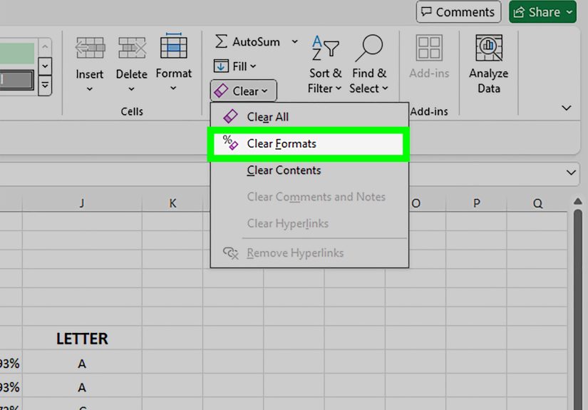
Clear formats (when things get messy)

If formatting has gotten out of hand, reset it:
Home → Editing group → Clear → Clear Formats.
This keeps your values but removes stylinglike taking off the costume without deleting the actor.

Troubleshooting: common “why is Excel doing this?” moments

Problem: I see ##### in a cell

Usually means the column is too narrow to display the value (especially dates/times).
Fix with AutoFit column width or widen the column.

Problem: My dates turned into weird numbers

Dates are stored as serial numbers in Excel. Change the cell’s number format to a Date style to display it properly.

Problem: Excel removes leading zeros

Format the cell as Text before entering the value, or apply a custom format like 00000.
This is especially important for codes, ZIPs, and IDs that shouldn’t be calculated.

Problem: My currency formatting looks inconsistent

Make sure the entire column uses the same format and decimal settings, and choose Currency vs Accounting intentionally.
Then verify whether negative numbers should display with a minus sign, parentheses, or red text.

Best practices: format for humans, not just spreadsheets

• Separate data from presentation: keep raw data clean, and format reports separately when possible.
• Be consistent: one date format per column, one currency style per report.
• Use styles for reusable formatting (headers, totals, inputs).
• Avoid merging in datasets: it causes issues with sorting, filtering, and copying.
• Let conditional formatting do the heavy lifting for highlighting rules-based patterns.

Conclusion

Once you know how to format a cell in Excel, your spreadsheets become easier to read, easier to trust, and easier to share.
Use quick formatting for everyday cleanup, the Format Cells dialog box for precision, cell styles for consistency,
and conditional formatting for dynamic insights.

The ultimate goal isn’t “pretty.” It’s clear. A well-formatted sheet helps people understand the story
your numbers are trying to tellwithout making them squint, guess, or accidentally interpret revenue as jellybeans.

Real-world formatting experiences: lessons from the spreadsheet trenches (about )

Formatting looks optional… right up until it isn’t. Most people don’t “fall in love” with cell formattingthey get
introduced to it during a crisis. Usually five minutes before a meeting. Usually while someone says, “Can you make this
look more professional?” in a tone that suggests professionalism is a button you forgot to click.

One common experience: someone builds a budget with clean formulas, but leaves the numbers as plain General format.
Then a total like 10000 sits next to 9500.5, and suddenly everyone starts debating whether the
decimals “mean something” or if Excel “did something weird.” A quick Number format with consistent decimals and thousands
separators ends the argument instantly. Not because it changes the mathit changes the confidence people have in the math.

Another classic: imported data. CSV files often arrive like a box of mixed cablesuseful, but chaotic. Dates may come in
as text, phone numbers lose leading zeros, and large values show up without separators. This is where formatting becomes a
cleanup tool. You set a Date format for date columns, apply a custom format like 000-000-0000 (or treat the
field as Text) for phone numbers, and switch currency fields to a consistent style. Suddenly, the same data becomes
readable enough that people stop asking, “What am I looking at?”

Then there’s the “accidental rainbow spreadsheet,” often caused by enthusiastic highlighting. Someone uses five different
fill colors, three font colors, and a border thickness that could qualify as architecture. The sheet becomes loud, and
the important parts are no longer important because everything is screaming. The fix is usually a calmer structure:
one style for headers, a subtle fill for input cells, and conditional formatting for the few things that truly deserve
attention (like overdue items or negative margins). When the noise goes down, meaning goes up.

Conditional formatting itself has a learning curve. It feels magicaluntil you inherit a workbook with 27 overlapping
rules applied to “the entire column forever.” In that situation, the experience teaches a simple truth: rules need
boundaries. Apply them to the right range, name or document what they’re doing, and use Manage Rules to keep things
predictable. Otherwise, you get the spreadsheet equivalent of a haunted house: cells changing color when nobody’s
looking, and you’re not entirely sure why.

The best formatting experiences are the ones you never noticebecause the spreadsheet just makes sense.
When numbers look consistent, dates display clearly, and important patterns pop without overwhelming the page,
people trust the sheet faster. And in Excel, trust is basically the highest compliment anyone can give you.